Simulating Slime Mold in Blender

There are two kinds of people: those who who are fascinated by slime molds, and those who don't know them yet.

Slime molds are single cell organisms and come in all sorts and sizes, with about a thousand species in total. Some of them are microscopic, while others like Physarum are macroscopic (meaning visible to the naked eye). I admit they do look a bit nasty, but when these little things crawl towards food, or away from light, their behavior is remarkably similar to that of way more complex organisms and even brains.

In a famous experiment, Tero et al. let a Physarium specimen crawl through a map replica of Tokyo, and the result resembled the city's railway network. Oh and also:

The filamentary structure of P. polycephalum forming a network to food sources is similar to the large scale galaxy filament structure of the universe. This observation has led astronomers to use simulations based on the behaviour of slime molds to inform their search for dark matter.
- Wikipedia

Simulating slime mold behavior isn't anything new (Jeff Jones wrote a paper about it in 2010), but it was something I hadn't done in Blender before. And when I read this amazing blog post by Etienne Jacob I'd have to give it a shot.

The basics

Before we dive into geometry nodes, let me briefly explain what's going on under the hood.

Our slime mold is represented by a set of particles that we simulate over time. To let patterns emerge, the particles need to follow two rules:

1. Each particle leaves a trail on the surface it is moving on. This is similar to the behavior of ants leaving pheromone trails. I'm going to call it trail density. New trails are added to existing trails (that means we are adding energy to the system).
2. Each particle moves in the direction of the highest trail density ahead of it.

To keep things stable, we also need to remove energy from our system, so we are going to diffuse and decay the trail density with each time step ever so slightly.

There are a couple of knobs we can later tweak to change the patterns of our little slime mold:

• How far ahead does it sense the trail density? This is our look-ahead distance.
• How far left and right does it look? This will be our sensing angle.
• How much momentum does it possess? When we update a particle's movement vector, we can mix it's existing velocity with the new movement vector.

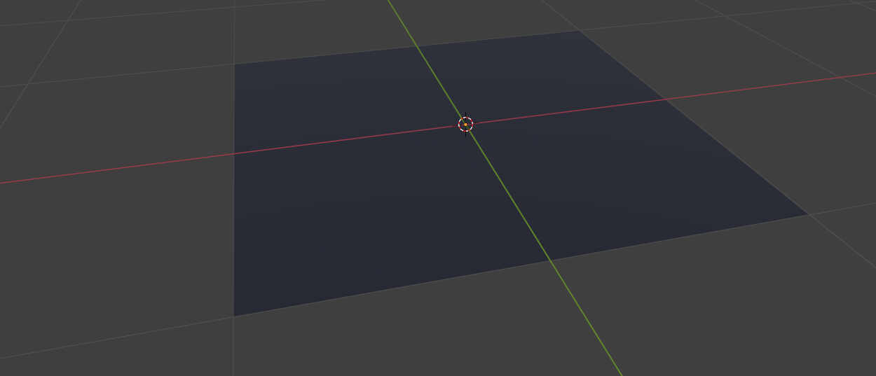
Flatland

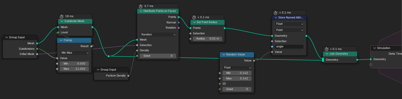
Most things are simpler to achieve in 2D, so let's start with a plane, subdivide it until we get a fine grid, and create a new geometry nodes graph for our simulation.

Our first task is to distribute points on this surface. We can expose the distribution mask to later play around with different initial conditions. We are also going to initialize an angle attribute for each of our particles. In this case, each particle gets a different randomized angle.

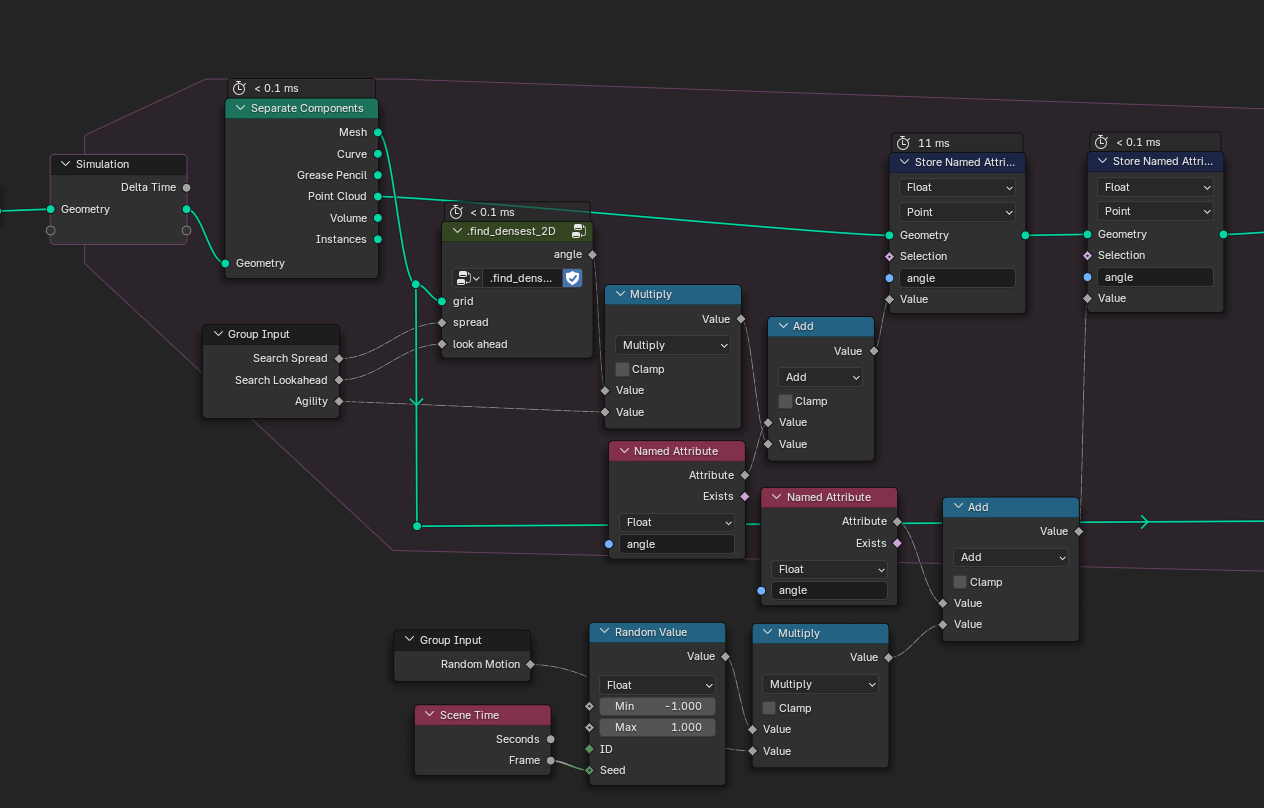
Inside the simulation zone, we need to work with both the particles and the surface mesh. That means we have to split the geometry into the mesh and the point cloud components at the start of each simulation step.

We then have to find the angle of highest trail density to update our particle's angle attributes. This happens inside the group called find_densest_2D. The resulting angle is then mixed with the existing angle. I also added a subtle random value to each particle's angle to spice things up a bit.

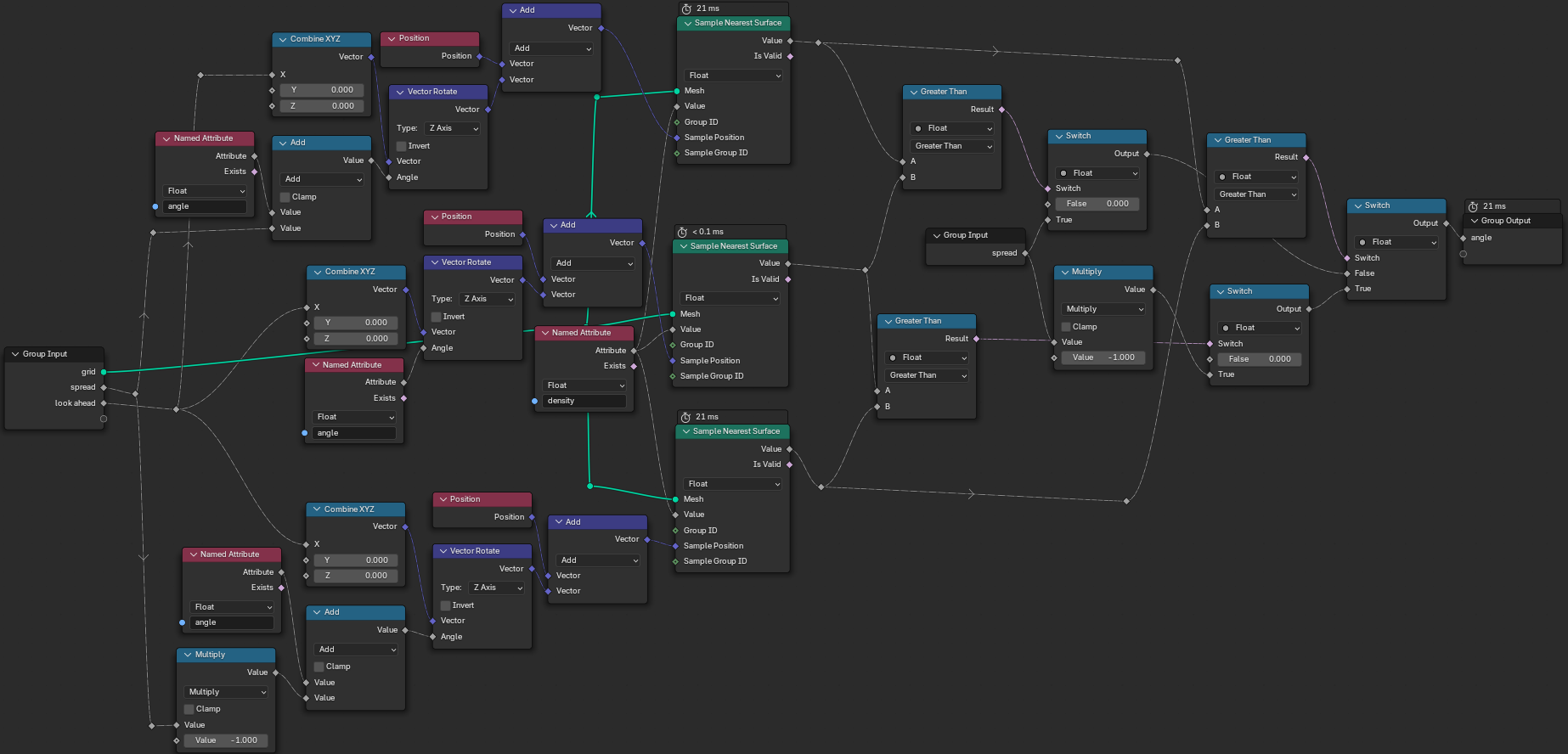
Now, what happens inside that group? We need to sample the surface three times. This is done with Sample Nearest Surface. The position we sample at is determined by the search angle and the look-ahead distance. Since we operate in flatland, we can simply use Z rotation to calculate our positions. With all three densities sampled, we lastly have to find the angle that corresponds to the highest density. For this I simply used three comparison nodes.

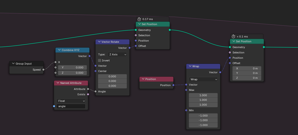
With our angles up to date, we can now go ahead and update our particle positions with the Set Position node. The magnitude of the position update is the speed at which our particles move. Let's expose it as an input to our node group. Since my plane is 2x2 meter wide, I decided to wrap the particle positions, letting particles emerge on the other side if they decide to leave.

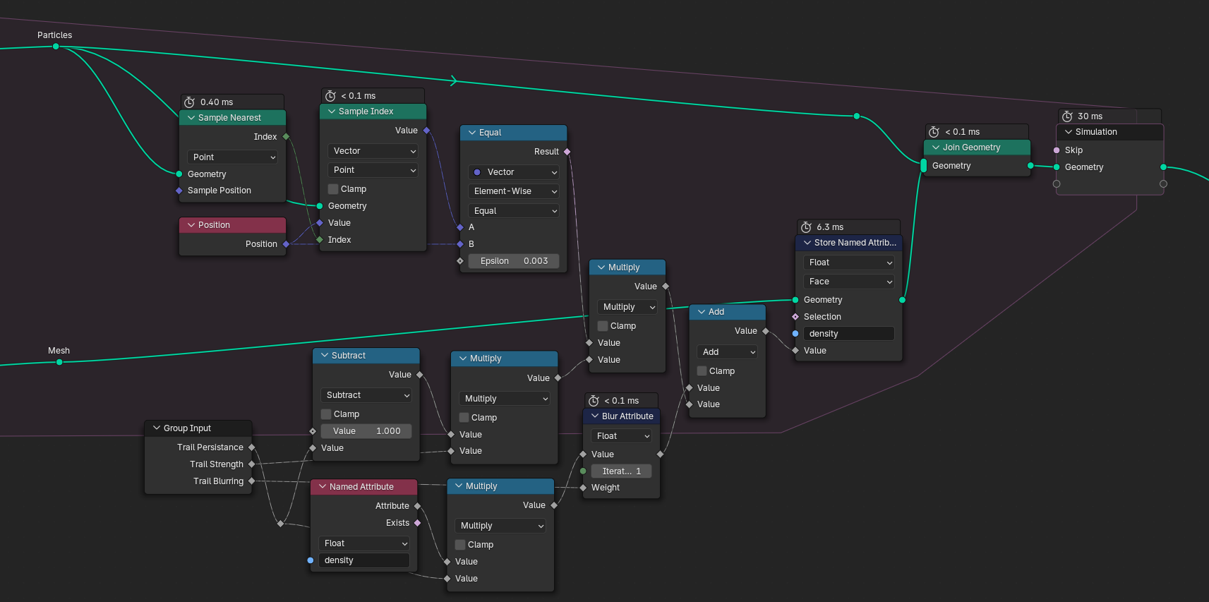
Let's recap: in the first step, we looked at our mesh to find the directions for our particles. In the second step, we updated the particle positions. Now for the third step, we turn things around and look at the particles to update the density of our mesh. All we have to do is combine Sample Nearest with Sample Index to get the mesh faces closest to the points and then add them to the density attribute. I added a few math nodes that take care of blurring and decay. In the end, we join both the particles and the mesh together again so we can pass it on to the next time step.

Here are some good starting values:

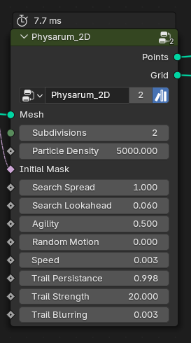
Search Spread is the half angle in radians in which the particle looks for the highest density. Which it does at a distance of Search Lookahead. Agility is a factor between 0-1 that states how much of the previous velocity is carried over (agility = 1 means no momentum). Trail Persistance should be kept close to 1, as it is the factor by which the field of density attributes is multiplied each frame. Something between 0.9-0.999 are good values. The higher your persistance, the higher the Trail Strength should be.

Let's have a look at the results:

To create these colors, simply add a new material and assign it to your plane with the Set Material node. Inside the shader nodes, access the density attribute using the Attribute node. You can then pipe it through color ramps, curves, etc, and drive the plane's diffuse color, emission or displacement with it.

Not too bad, right? But how about we take this a step further and move into...

The Third Dimension

Bad news: we can no longer represent particle directions as a simple float value (do I hear "oh no!" cries?). That's right, we're now dealing with 3D surfaces, and this comes with a couple implications. We have to:

• represent particle velocities as vectors (I'm going to call those vel)
• find a way to perform the look-ahead density sampling on a complex 3D mesh
• update our particle positions so they always move tangentially to the surface

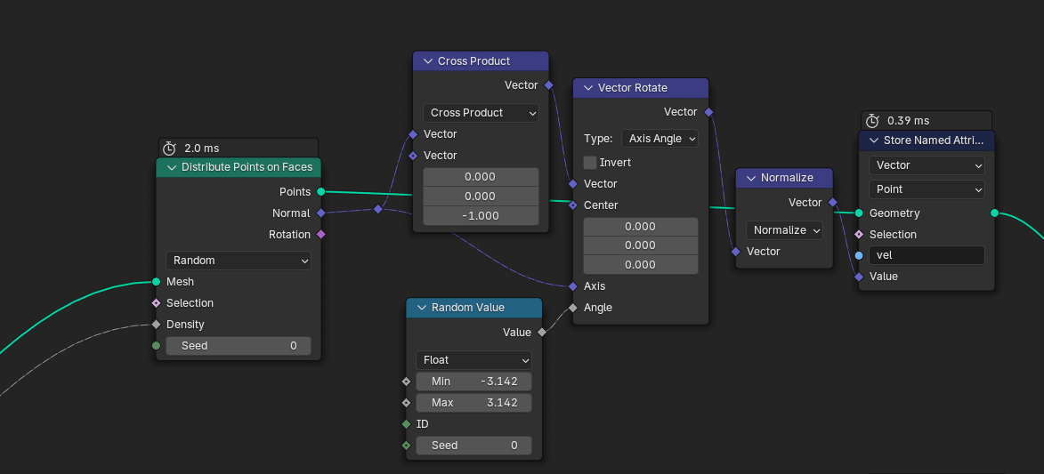
For starters, we can't directly use a random vector as initial velocity. Instead, we take the cross product between the surface normal at the particle's initial position and the downwards vector. This gives us a tangent vector that we can rotate randomly with the surface normal as rotation vector.

Entering the simulation zone.

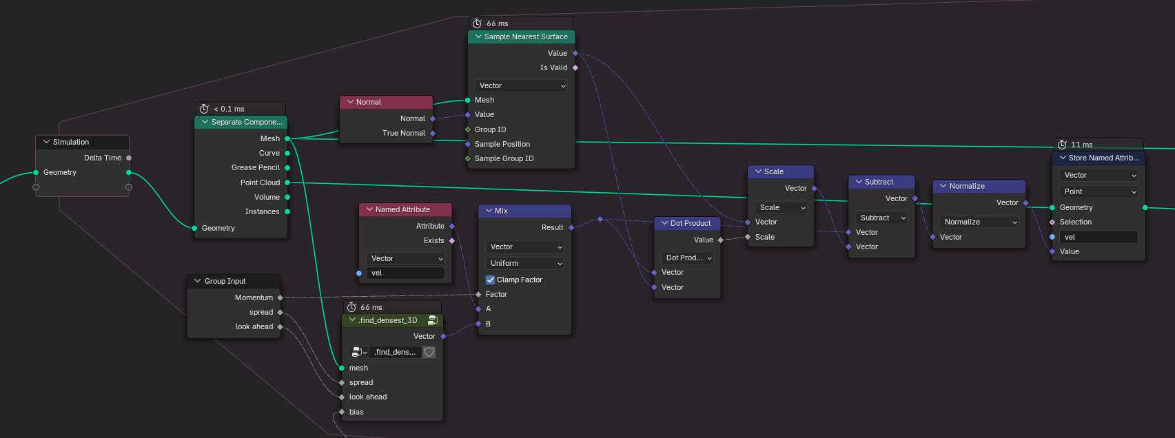
Let's find our angle with the highest density. We can keep our group from flatland, and only change the sampling to this:

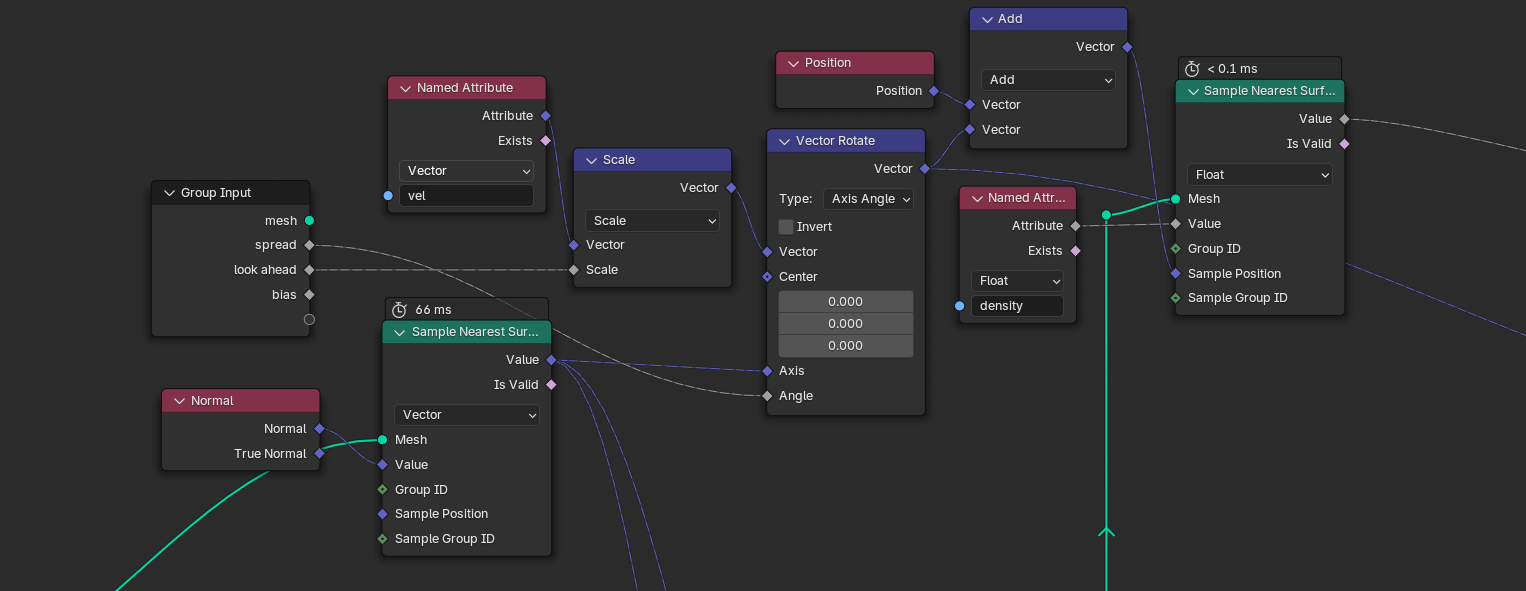
Since we can no longer use the search angle directly, we instead rotate our velocity left and right with the mesh normal as axis, similar to what we did for our randomized initial directions.

Updating our velocity now becomes a little more involved. Time to activate our last brain cells and think about this for a second:

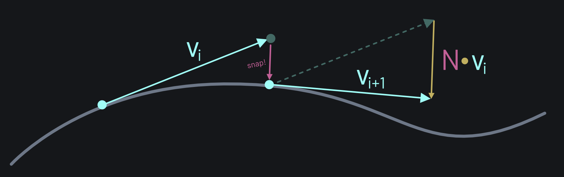
Here, Vi is our current velocity. After moving the particle and snapping it back to the surface, we'd end up with a velocity that is no longer tangential to the surface. The dotted vector has two components: the new tangential velocity vector that we'd like to store (Vi+1), plus a non-tangential component. We can compute this component as the dot product between surface normal and Vi. To get Vi+1, we simply subtract N∙Vi from Vi:

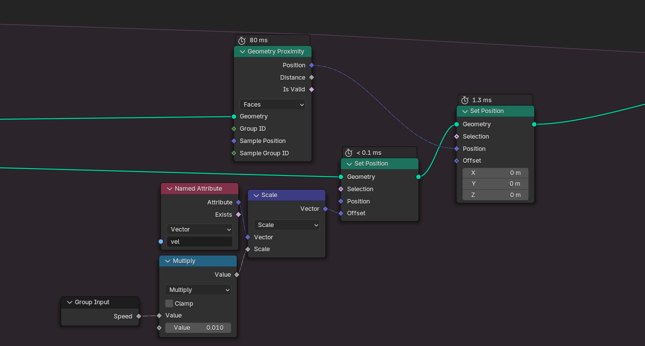
Updating the particle positions is almost as easy as before. All we have to do is snap the particle to the closest mesh position:

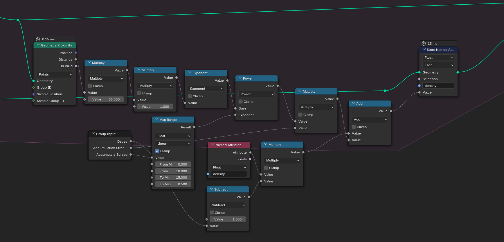
Updating the density stays the same too. Instead of doing a hard comparison between particle and mesh positions, we can smooth things out with an exponential falloff function:

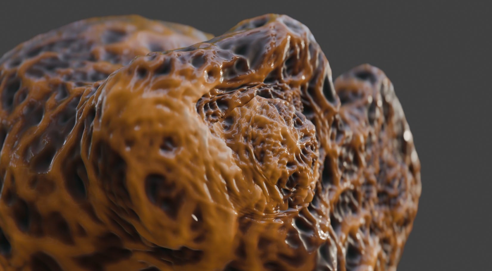
Time to see some results!

For these videos, I used the density attribute in several ways: it drives the mesh displacement, it influences the color and also the roughness.

And that concludes our little slime mold adventure. If you got any questions about this tutorial, feel free to reach out to me on Mastodon, or leave a comment under this article with your favorite ActivityPub client (because this blog is federated).

You can find the blend files for this project as free download here.