Tutorial: Diffusion Limited Aggregation in Geometry Nodes
I recently had the chance to meet the great Andy Lomas on a conference, and his custom CUDA code for simulating cell growth and diffusion limited aggregation processes sparked the idea in me to explore this concept in geometry nodes.
Diffusion limited aggregation essentially works like this:
- Start with a seed structure
- Spawn particles that follow brownian motion (and/or are driven by a vector field) until they hit the seed structure, where they attach to it
- Spawn more particles, and grow the structure further.
The idea was first explored by Witten and Sander in 1981.
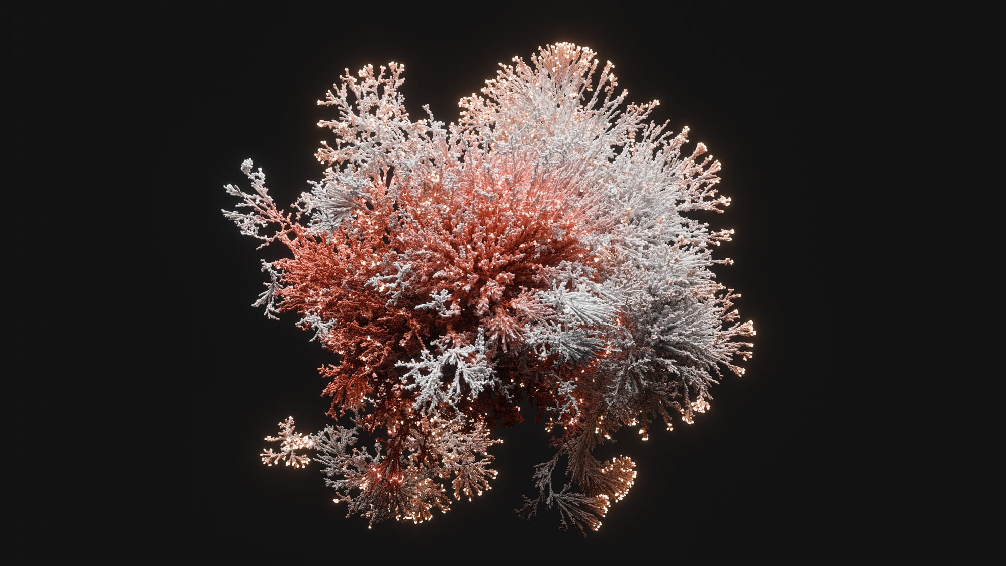
By manipulating the vector field that influences the particles, its possible to grow all kinds of structures. Each of the following structures is made up of around 2-4 million points, directly rendered as point clouds in Cycles. Past that point, Blender crashes because it can’t fit more into my VRAM.
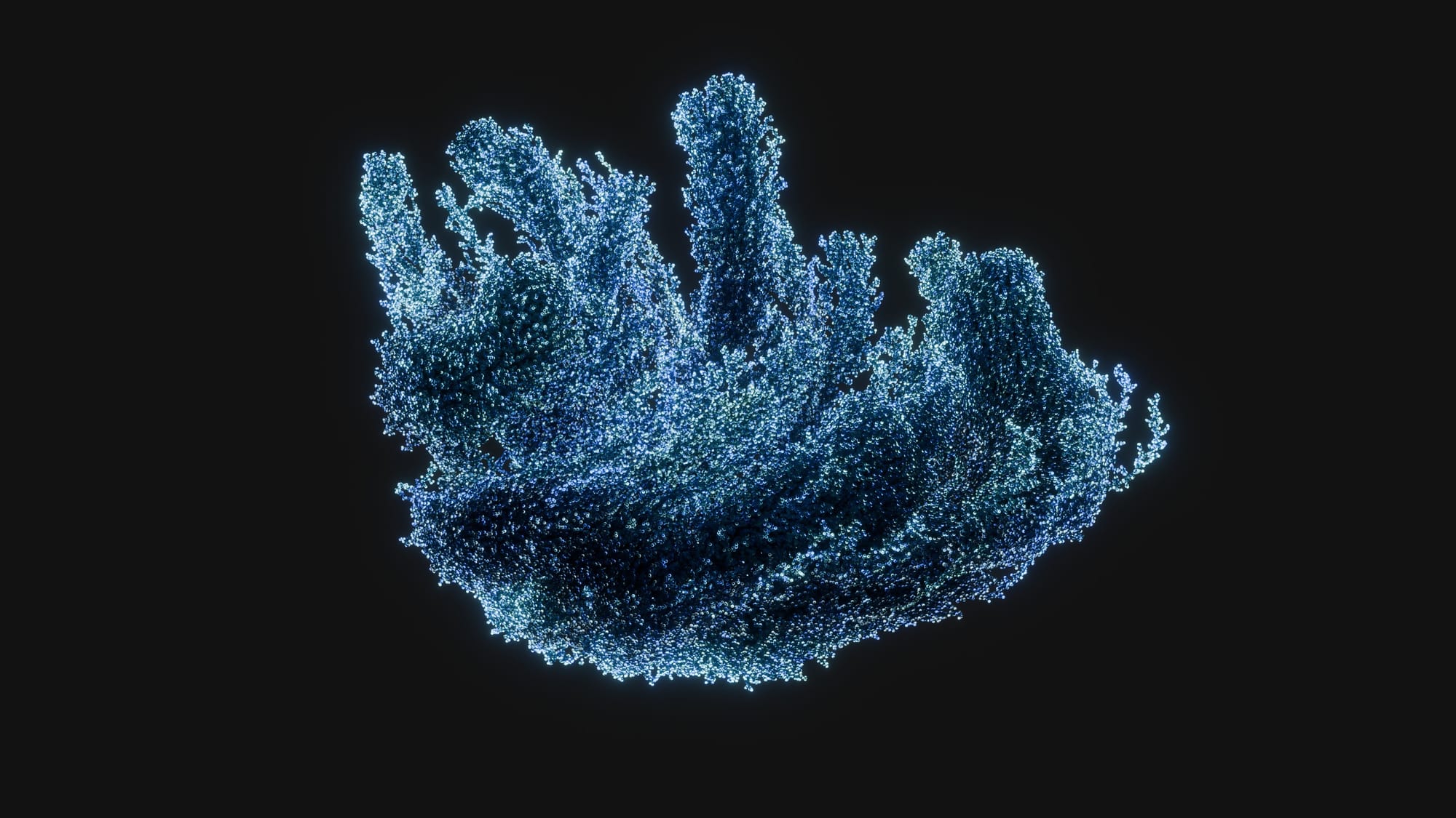
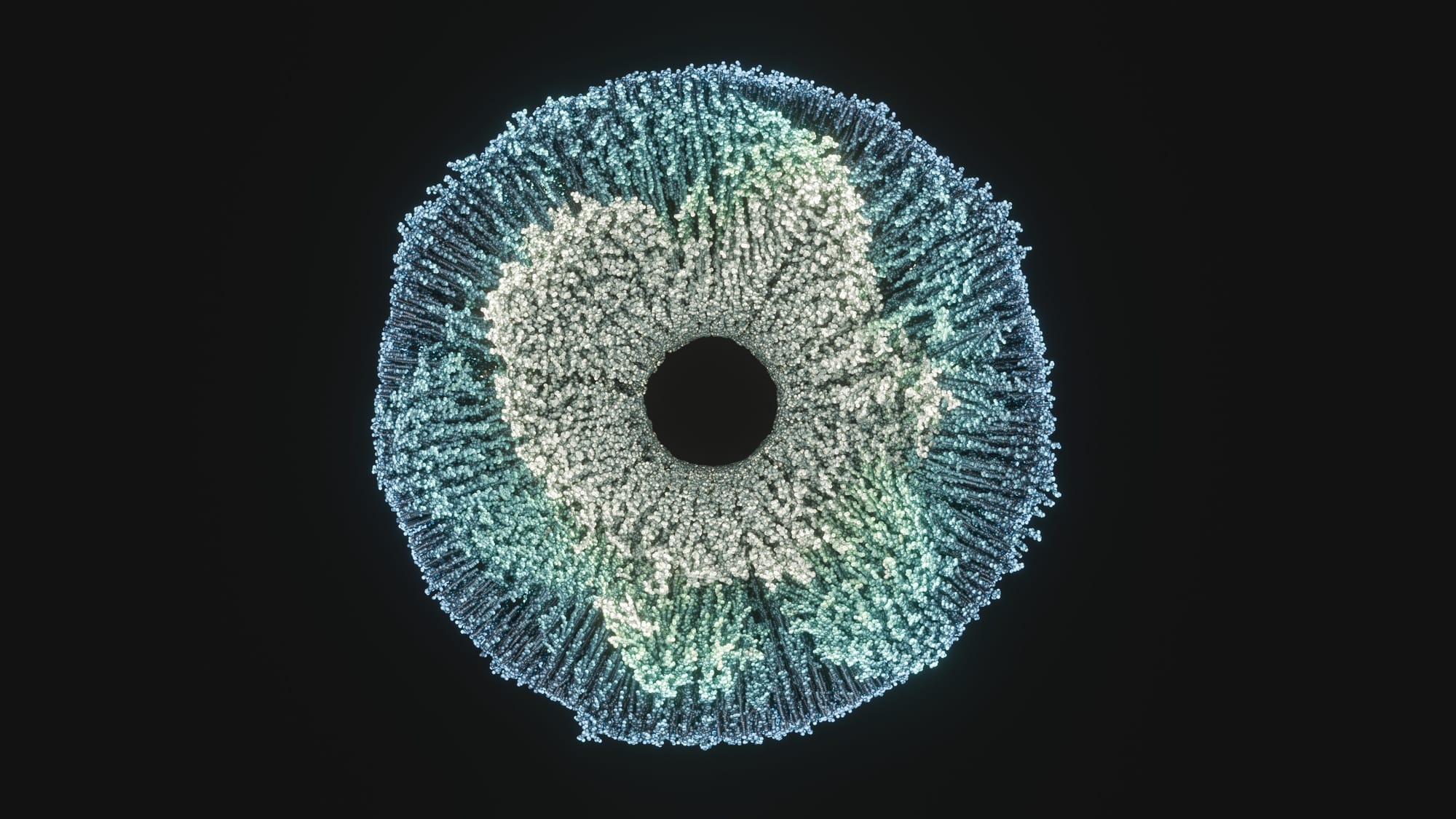
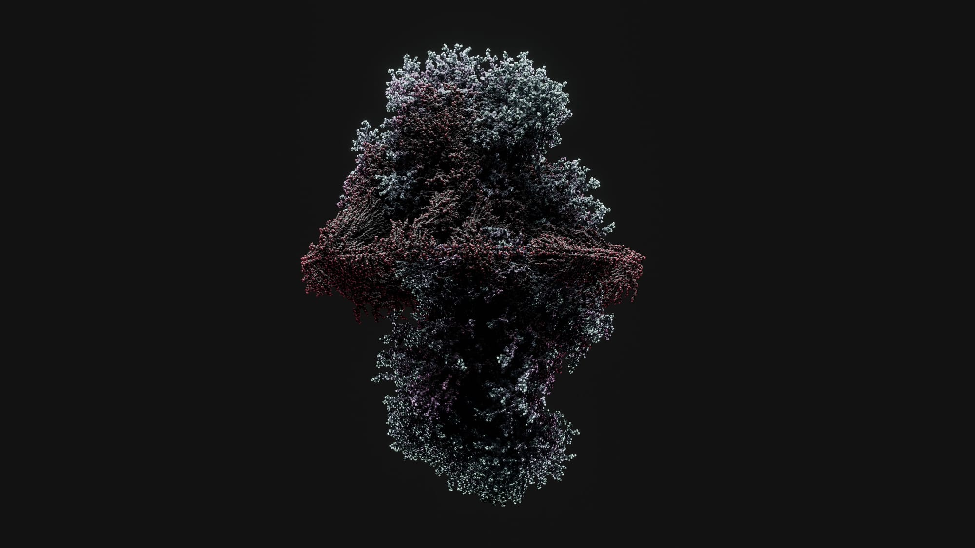
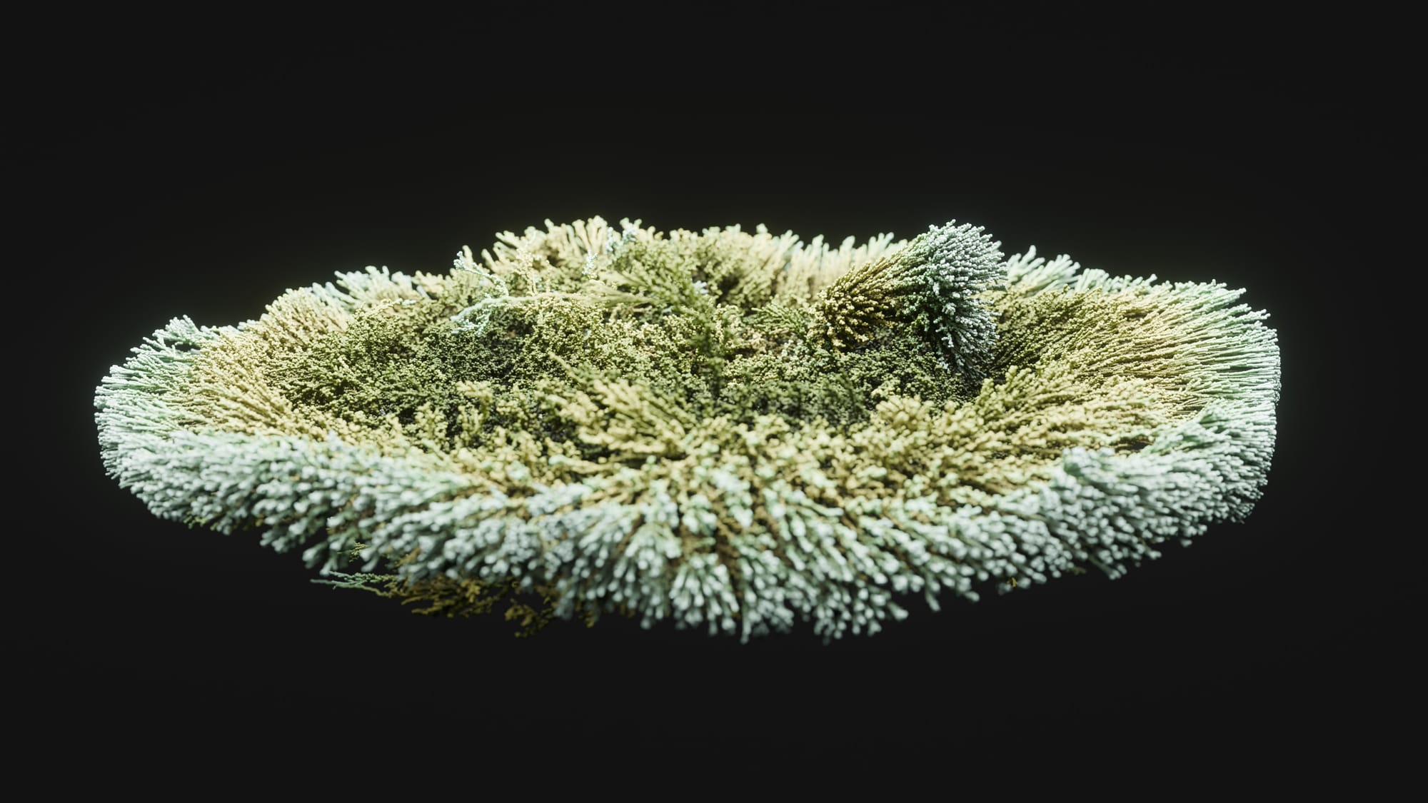
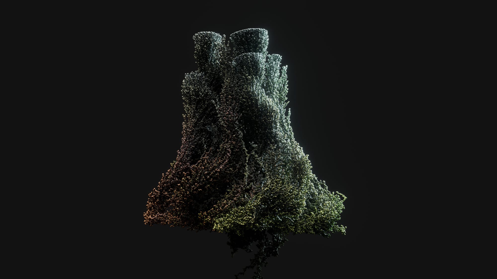
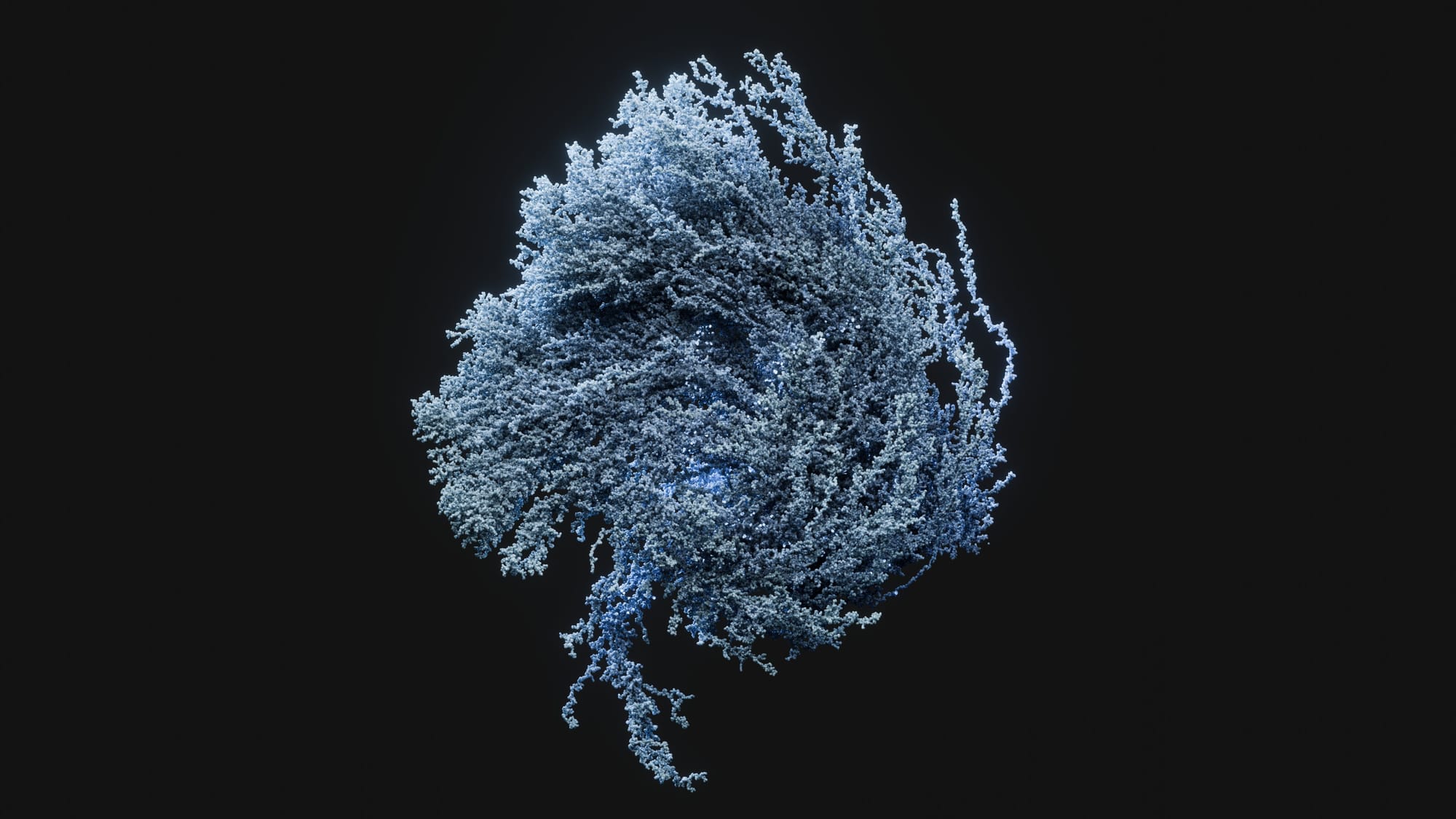
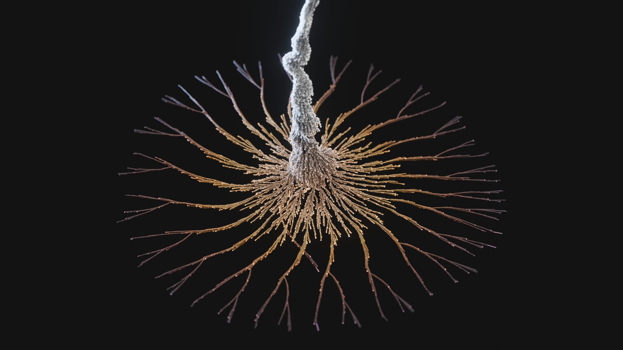
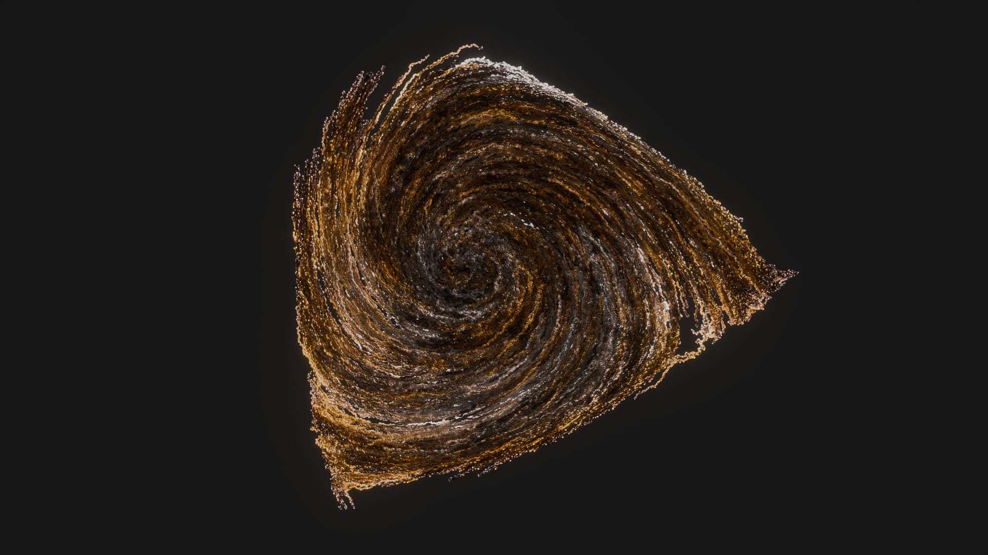
Variations in the flow field and movement simulation lead to a variety of fascinating structures.
Animation
Soundtrack and SFX by me.
How to DLA
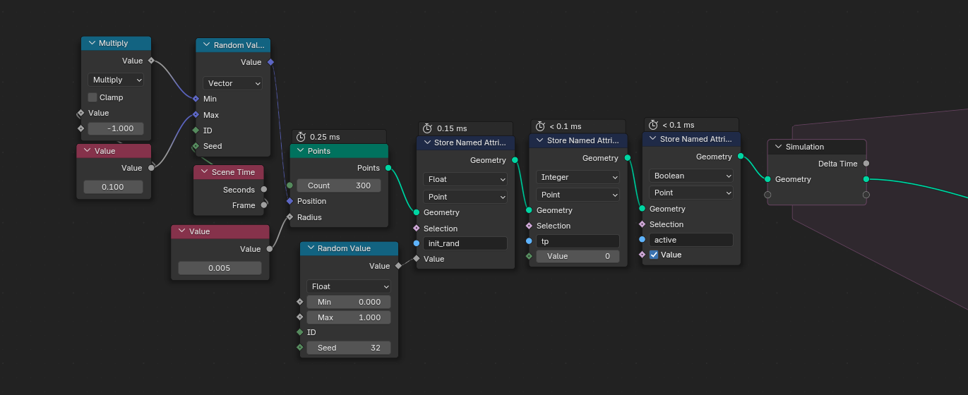
Initialization
Before we hop into the simulation zone, we have to initialize a few points that act as our seed structure. Here I chose a few randomly displaced points, but I also experimented with using simple base geometry and then distributing points on its surface. I also capture a few attributes here that will help us with driving the shader colors (i.e. an initial random color and the timepoint of the particle), as well as a boolean flag that determines whether the current particle is active or not (meaning whether it is part of the fixed structure or still floating around).
Simulation
The simulation itself is fairly simple:
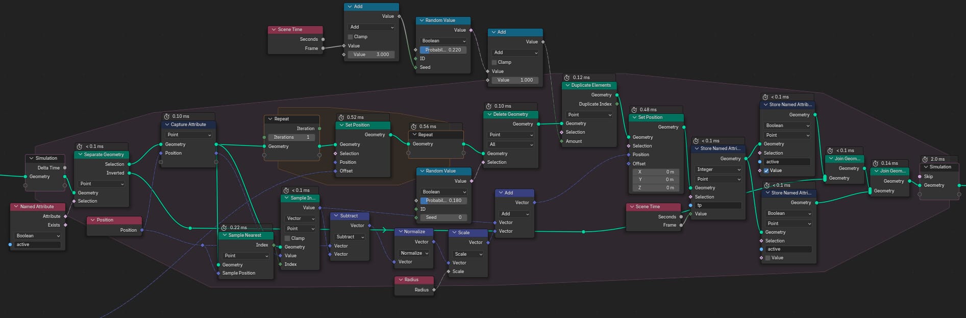
I first split the active geometry (aka the moving particles) from the fixed structure (where active = false). The active particles are then displaced inside a repeat zone based on the rules given by the flow field (see following section). Tweaking the amount of repetitions will give you increased particle movement and randomness.
After the points are displaced, there is a chance that the particle is deleted; this helps with fighting exploding complexity, as I duplicate the particle with a certain probability in the next step. Both the duplication and deletion chance have a big effect of the sparsity of the structure.
Next comes a little hack. In a naive implementation, you’d simulate the brownian movement of all active particles over time until they touch the seed structure or until they exceed a timeout. This is not really practical for a geo nodes implementation, where I’d like for each timepoint to deposit one layer of particles, so instead I do the following: After moving the particle around, I snap it to the closest seed structure. This is done by sampling its nearest index and position attribute, then getting the normalized directional vector from particle to the sampled position and then snapping it to the structure with a distance offset of one particle radius.
The interested reader might have noticed that the position that I sample is in fact not the seed structure, but actually the active particle before it is displaced by flow field and brownian motion. This is technically not quite correct, but it accelerates the simulation significantly (and it looks close enough, so its whatever). The reason for this is that the number of active particles is always way smaller than the total number of particles in the structure. Sampling only from this small active subset is obviously a lot faster, and before we displace the active particles, they share their position with the fixed structure (as they were put there in the previous time step).
To deposit the active particles, I attach two copies of them (with active = true and active = false) to the structure (using the Join Geometry node). One to remain part of the structure, the other copy to become the active particles for the next iteration.
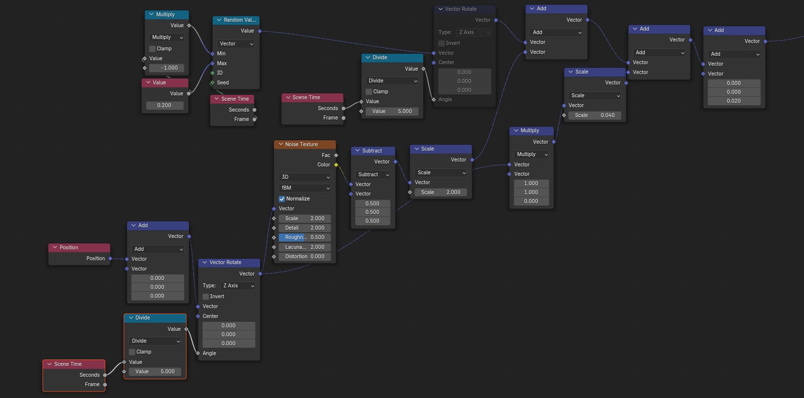
Flow field
This part drives the displacement of all active particles inside the repeat zone, and the nodes here are a messy playground of different factors that I switch on and off to see what happens. This includes brownian (meaning: random) motion, rotation around the Z axis, a 3D noise texture to let large scale structures emerge, a small factor for movement towards the positive Z axis (i.e. plant-like growth), or factoring in the particle’s current position to allow for global outwards or inwards movement.
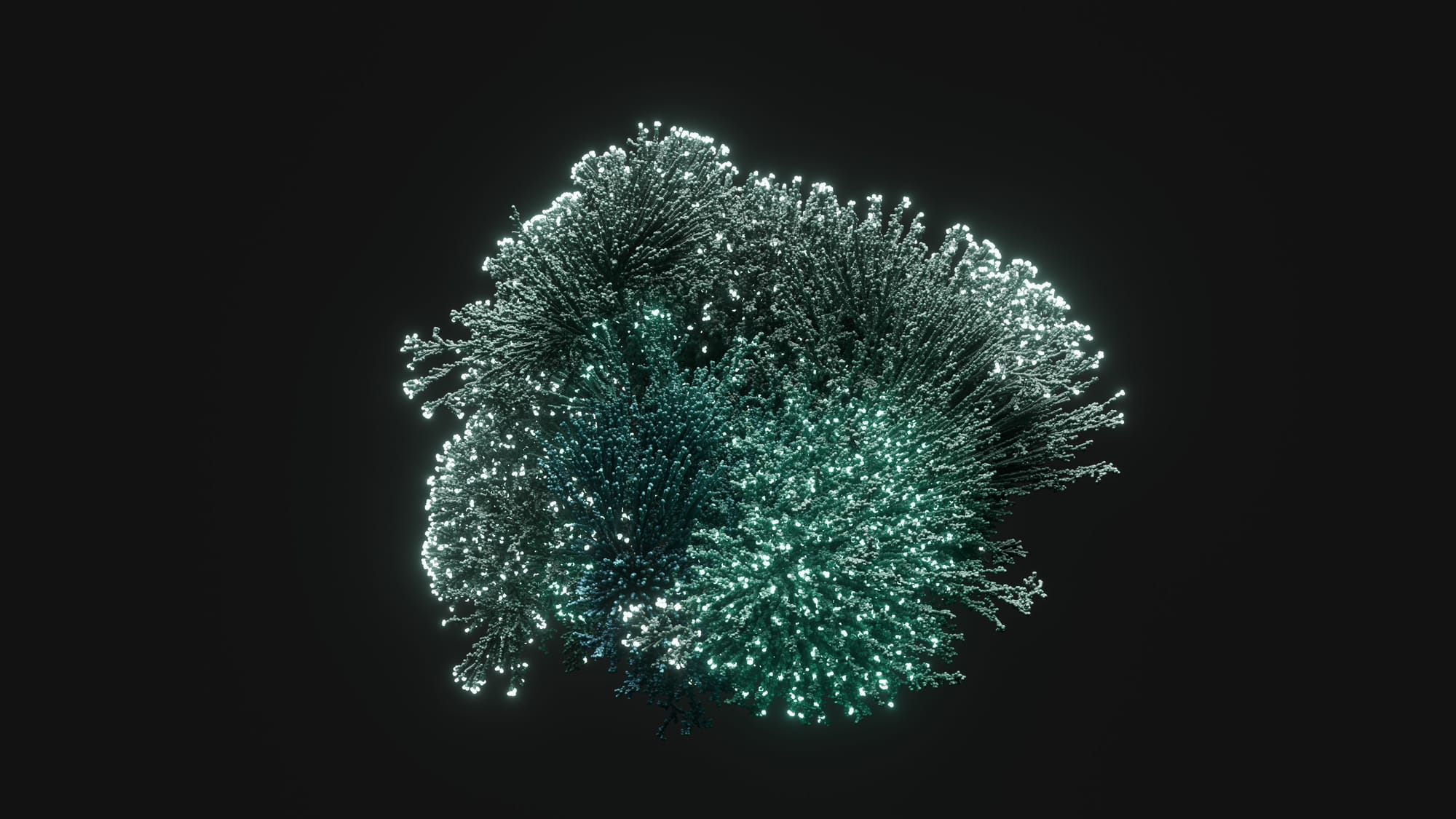
Material
We captured a few attributes in the simulation that we can now use for coloring the structure. This can be the initial random values that we captured for each seed particle, or the timepoints. If we divide the timepoint attribute by the current frame number, we get a range from 0-1 that allows us to create a color ramp. Another way to utilize the timepoint is to compare the timepoint attribute with an arbitrary integer value and use the resulting boolean to drive an emission shader. This way, we can let the ends of the structure emit light. Or any particle, for that matter.
Another way to create interest in your material is to mix in the Ambient Occlusion node, either with default setting or with inside = true.
I also posted this tutorial over on Blenderartists.