Creating a Pipe Generator in Blender

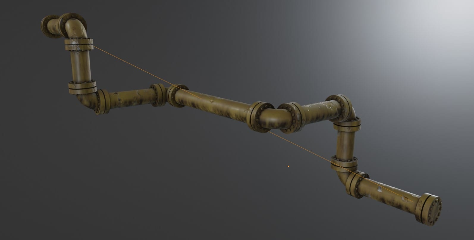
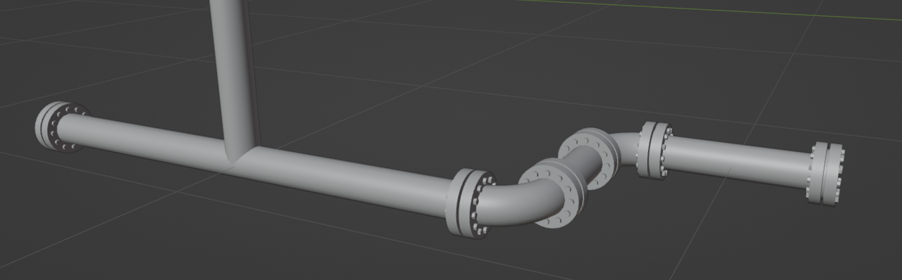
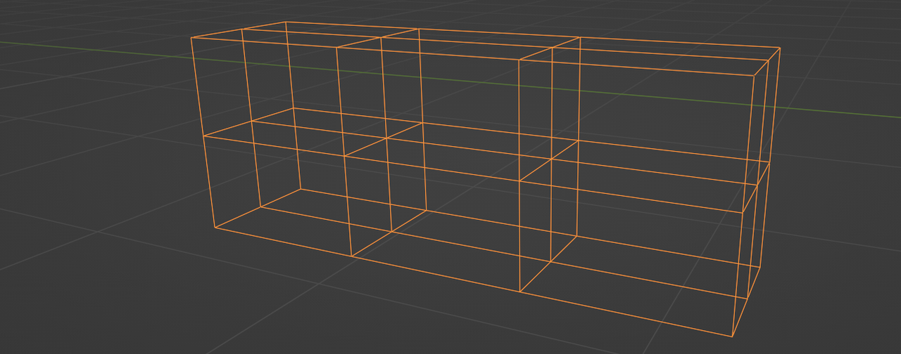
Pipes are complex objects and add realism to any 3D scene (unless you are modelling an animal, I guess), yet they can be quite tedious to model manually. Thanks to the power of Blender's geometry nodes system, this is a task we can automate with ease. In this tutorial I'm going to walk you through the basics of creating a pipe generator. The goal is to use basic mesh edges as input (very easy to draw), and the generator will turn them into pipes that follow a 3D grid-like structure with automatic path finding, randomized offsets and adjustable junction pieces.

Water to wine, edges to pipes

Any complex problem becomes easy once you break it down into smaller problems that you can solve. So let's start with the basics: we need a node group that can turn any input edge into a pipe. Once we have this set up, we can later build upon it by adding the fancy stuff like path finding and special treatments for junctions.

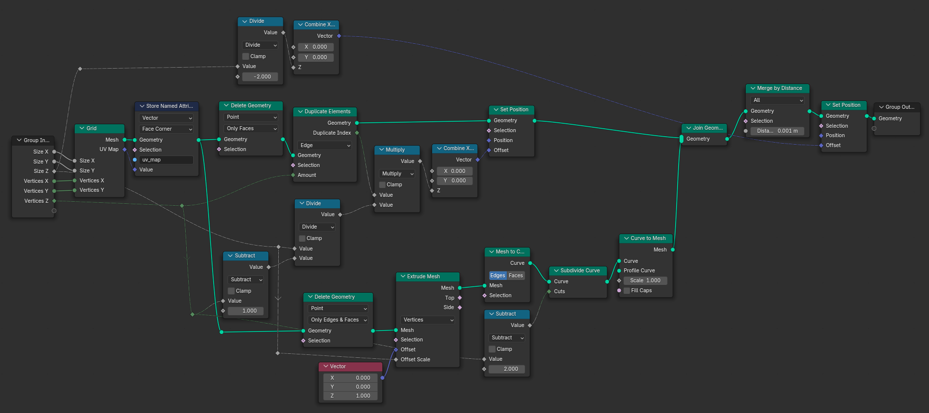
The first thing to consider is rounding the curves. No pipe has straight corners, so we need to find a way to fillet them. Luckily there is a curve node that does just what we need: Fillet Curve. Before we can do that though, we'll have to convert Mesh to Curve, considering our input consists of a simple mesh. But we only want to fillet the corners, so we have to check whether the two edges are actually parallel to each other or not. This is where your vector math knowledge from school will come in handy: we're using the dot product of both edge directions. If the dot product is 0, the vectors are in a 90° angle to each other, if it's 1, they're parallel. We can use the Field at Index position of the current index, the index -1 and the index +1 to compare two adjacent edges:

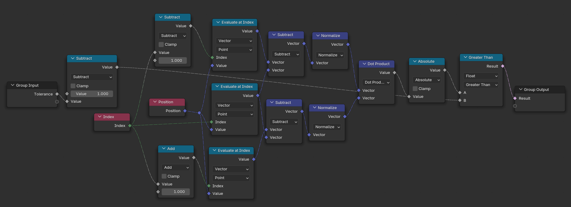
If the two edges are parallel, we can set the Fillet Curve radius to 0.

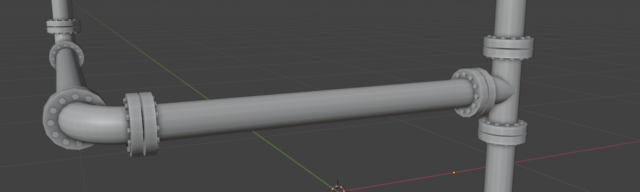
Once this is done, there are two steps left for a basic pipe: turning it into a 3D mesh, and adding the flanges. The first step is easy: simply use Curve to Mesh with a Curve Circle as profile. Adding the flanges is a bit harder. Let's assume we already created some sort of flange object – e.g. a simple cylinder. How do we determine on which points of the curve to instance that flange? There might be better ways, but I used the Attribute Statistics node with the edge length as input. We can assume that the tiny edges added by the filleting step are the shortest edges of the pipe, as well as the most common length, statistically speaking (unless you reduce the filleting resolution by a lot). We don't want to instance on the filleted corner vertices, only on the others. That means we have to create a selection where every edge larger than the median length is considered for flange instancing (for which we can then use the Instance on Points node). To that selection we add every vertex that has only 1 adjacent vertex. Why? Because we want the start and end points of our pipe to get flanges, too.

Now, how do we find the correct direction in which to rotate the flanges? By simply capturing the curve tangent for each point of the input curve and passing them to the Instance on Point's Rotation input via an Align Rotation to Euler node.

From 3D lattice to paths

Now that we have a node group that turns every edge we throw at it into a pipe, it's time to start with the cool stuff: creating grid-like paths on our input edges.

We can create these orthogonal paths with the Shortest Edge Path node. In conjunction with the Edge Paths to Curves node, we can pass selections for both the end vertex and the start vertices to the path finding algorithm, which then tries to find a path through an arbitrary mesh to connect these vertices with respect to an edge cost function. That leaves us with two questions: how do we create a 3D lattice mesh around our input edges which the Shortest Edge Paths node can work on, and what do we use as edge cost function?

To create a 3D edge lattice, we simply start with a 2D grid with the given X and Y dimensions and duplicate it upwards along the Z axis. The amount of subdivisions and duplication along the Z axis depends on the lattice resolution we need; I created a parameter that controls this resolution. As a last step for a basic 3D lattice we need the vertical edges: we instance upward-pointing curve lines on every vertex of the bottom-most grid, and divide the curve lines by the amount of grid rows on the Z axis. This subdivision step is required so we can use the “Merge by Distance” afterwards, which merges all vertices together.

Now that we have a generic 3D lattice, lets make it adapt to our input geometry. To do that, we use the Convex Hull node on our input geometry; it creates an enclosing mesh around all our input edges. We can then use the statistics of the positions of the convex hull vertices to change the scale of our 3D lattice and its offset in 3D space (in retrospect, the Convex Hull might even be redundant). For that, we use the Range and Minimum values of the Attribute Statistic node:

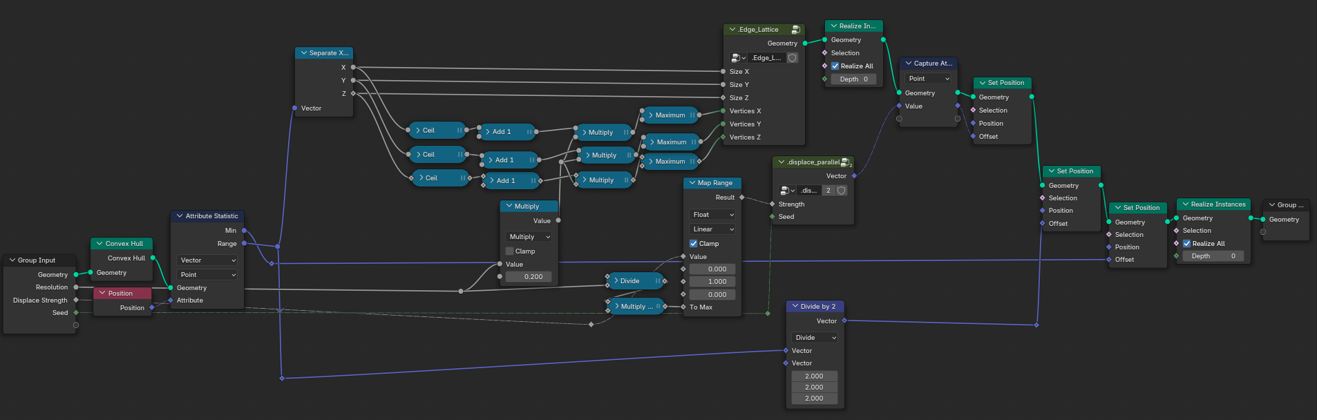
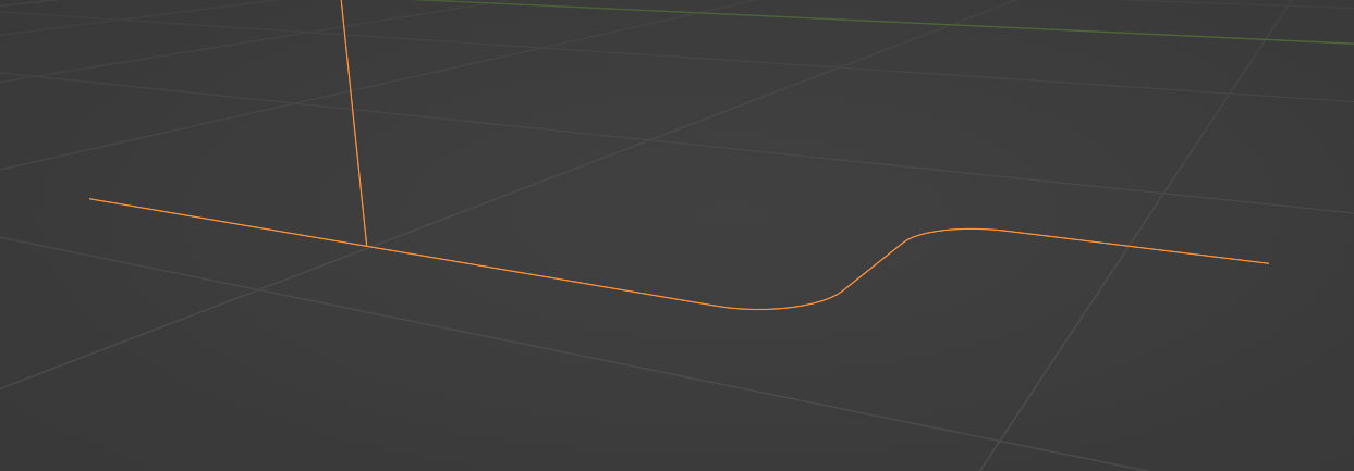
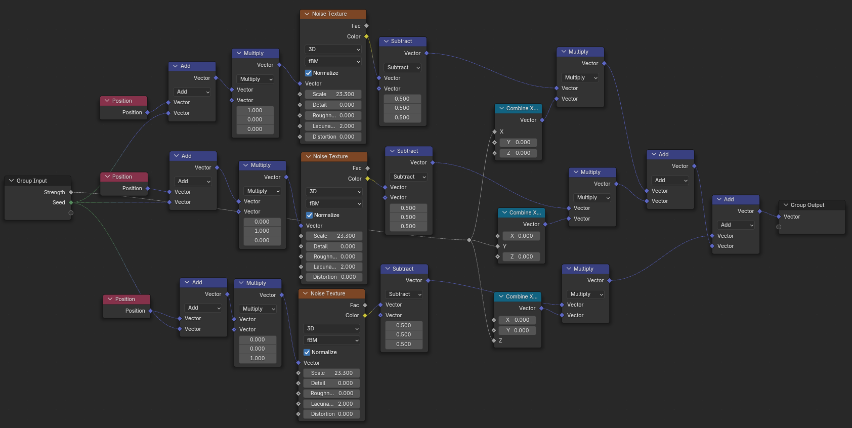
To break the repetitive pattern of the lattice, we could offset the edges in random directions. But what happens if you offset a single edge of the lattice in a random direction? The adjacent edges will rotate and break the orthogonality of the lattice. To fix this, we have to move every row of each dimension as a whole. That means every edge in the X-Y plane would have to move in a random Z direction. To get a random value per row, we can use a noise texture with a one-dimensional vector as its input vector. Lets take the X dimension as an example. Our noise texture will only change in [1, 0, 0] space. We do the same for the other dimensions and combine them to a unified vector value (because its easier to pass on). We then capture this vector for every point on the lattice and let it drive the offset of the “Set Position” node. And et voilà, our lattice is no longer repetitive.

Time to move on to the Shortest Edge Path. How do we tell the path finding algorithm where to start, where to end and where to draw the paths? To do that, we transfer the positions of our input edge's start- and endpoints with Sample Index to the Sample Nearest node that takes these positions and transfers them to the 3D lattice as its input geometry. The resulting selection contains the nearest vertices in the 3D lattice corresponding to the start- and endpoints of our input mesh. Sounds complicated? Let me show you:

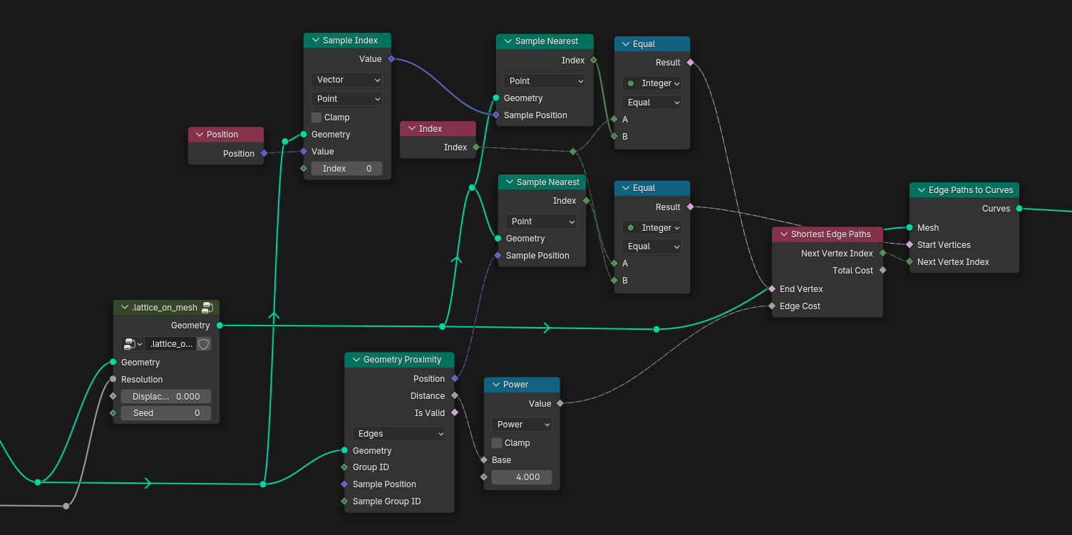
Now what about the edge cost? We simply use the distance value of the Geometry Proximity node to drive the edge cost, as seen above. The farther a lattice edge is from the input edge, the less likely it is to be used by the path finding algorithm. You can increase the falloff speed by running the distance through a power function.

Junctions

I'm not a plumber, but I think whenever a pipe splits up into two sections, there needs to be a junction piece. How could we add this to our existing node graph? We already have a group that adds flanges at the end vertices of edges, so why not use that to our advantage?

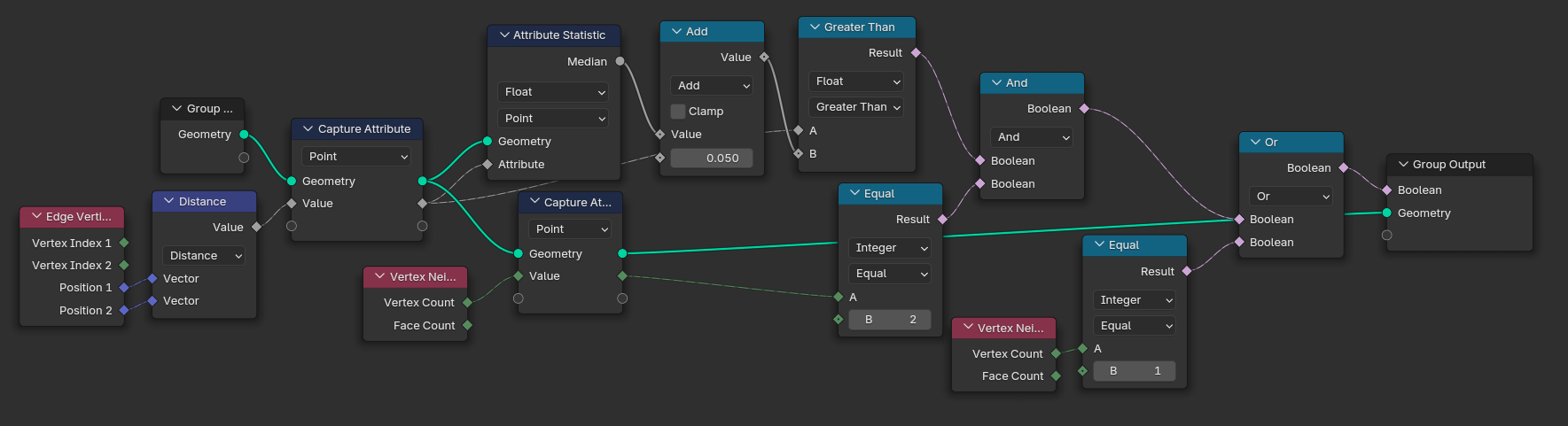
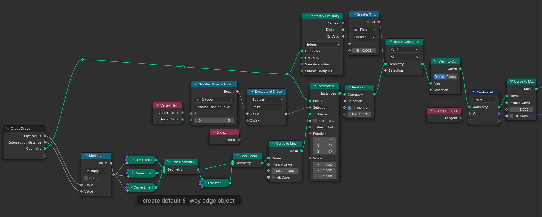
First we have to select all junction vertices. Those can be found by checking the number of vertex neighbors for each vertex (if there are more than 2, we found a junction).

The most elegant way would then be to spawn N lines on each junction vertex, where N is the number of adjacent junction edges, and then capture the directions of said junction edges and rotate the instanced lines accordingly. This would give us new endpoints to spawn flanges on, and they'd be spaced evenly from the junction center. I tried that ... and it didn't work, because I couldn't find a way to tell the node gods which rotation belongs to which instanced line; their indices are completely different from the indices of the junction edges.

So back to the scratch pad we go. What if we simply create a 6-way hedgehog of lines (one for each orthogonal direction; +/-X, +/-Y, +/-Z) on every junction vertex and then delete those of the lines that don't overlap with the pipe? Using the distance of the Geometry Proximity node, we can drive a Compare node and create a selection. Each of the hedgehog lines (what a silly name) whose distance is bigger than close to zero gets deleted. What remains are lines that align with our existing pipe paths and have a defined distance to our junction vertices. Of course this only works as long as the paths are orthogonal to each other, but its better than no junctions at all, I guess.

Conclusion

So there you have it, this is how I created my pipe generator. I had to cut a lot of corners in my explanation (or should I say, filleted?) but I hope you get the general idea of what's going on and could learn a thing or two about working with Geometry Nodes. If you want to try out the generator yourself or dissect my node graph, you can grab an extended version here on Blendermarket for a few bucks. It contains several procedural materials and a few advanced bells and whistles like spawning multiple randomized pipes at once. Happy blendering!